


TL;DR: Accounts receivable forecasting predicts when the cash your customers owe you will actually arrive. Forecasts built on invoice due dates are the most common and the least reliable, because more than four in ten B2B invoices are paid late. Forecast from how your past billing months really collected, check the error every week, and the forecast becomes a number the board can plan against.
Accounts receivable forecasting: how to predict cash receipts you can plan against
Accounts receivable forecasting is the practice of predicting when your open invoices, and the invoices you are about to issue, will turn into cash in the bank. A good AR forecast gives you a dated view of customer receipts for the next one to six months, built from how your customers actually pay rather than from what their payment terms say.
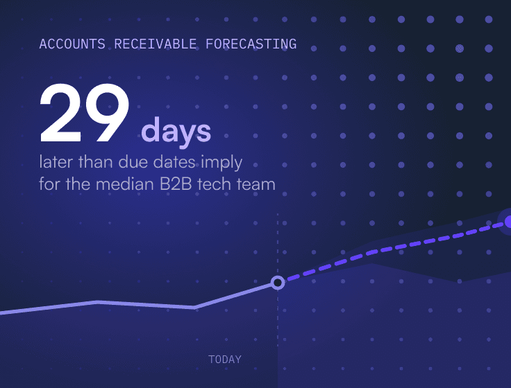
That distinction is where most forecasts go wrong. In Upflow’s benchmark research across thousands of B2B tech finance teams, the median company runs a DSO of 52 days against a best possible DSO of 23, so cash arrives 29 days after the date the terms imply. A forecast built on due dates bakes that gap into every line. This guide covers the six methods finance teams use, where each one breaks, how to build a cohort-based forecast in a spreadsheet, and how to tell whether it is any good.
What is the difference between an AR forecast and a cash flow forecast?
An AR forecast predicts one line of the cash flow forecast: cash received from customers. The full cash flow forecast adds payroll, supplier payments, tax, debt service and financing. Customer receipts are usually the largest and least certain inflow, so getting them right does most of the work.
Two different questions also hide behind the phrase “forecast accounts receivable”. FP&A teams building a three-statement model often mean the AR balance at month end, projected as receivable days multiplied by forecast revenue. That tells you how much will be owed. It says nothing about when the cash lands, and timing is what a CFO managing runway actually needs. This article is about timing.
Why do AR forecasts go wrong?
AR forecasts usually fail for four reasons: they trust due dates, they give overdue invoices no date, they ignore disputes, and they run on stale data. The symptom is the same each time, a forecast that looks fine for next week and drifts further from reality every week after.
Due-date optimism is the big one. Atradius’s 2025 US Payment Practices Barometer found that overdue invoices affect 43% of credit-based B2B sales in the US, on average terms of 45 days. In Western Europe the figure is 47%. A method that assumes every invoice clears on its due date is wrong on close to half the book before it starts.
Overdue invoices are the second trap. Once an invoice passes its due date, a due-date model has nowhere to put it. Some teams drop it, which understates cash. Others assume it arrives this week, every week, until someone notices the same 200k has been forecast for six weeks running.
Disputed invoices will not pay until the dispute closes, however many reminders go out. And the data underneath is often worse than it looks. PwC’s 2025 Global Treasury Survey of 350 treasurers found poor data quality was the most cited obstacle to better forecasting, named by 76%. Unapplied cash in a suspense account looks exactly like an open receivable, so a messy ledger will forecast cash you already have.
The AFP’s 2026 Treasury Benchmarking Survey names cash and liquidity forecasting as treasury’s most frequently cited challenge, at 49% of respondents.
What are the main methods for forecasting accounts receivable?
Six methods are in common use, running from simple and fragile to data-hungry and precise. Most B2B tech companies should run a cohort curve as the base forecast, then layer promises to pay and customer-level detail on the few accounts large enough to move the total.
1. Invoice due dates
Every open invoice is forecast to arrive on its due date. The only input is an aging export, which is why it is the default in most ERPs and spreadsheets. It breaks on overdue invoices, on customers who routinely pay 15 days late, and on anything not yet invoiced. It suits a small book of reliable customers and little else.
2. Expected payment dates and promises to pay
The AR team replaces the due date with a date the customer has given: a promise to pay, a payment run, a remittance advice. For the next two weeks it is the best input you will get. Promises slip, though. Upflow’s book From Zero to Collected lists promises kept as a live signal to review weekly, and that rate tells you how much weight each promise deserves.
3. DSO-based projection
You assume receipts equal sales from DSO days ago. HighRadius sets out a three-step version: forecast sales, calculate DSO, multiply. It breaks because DSO is one average. A book where half the customers pay in 20 days and half in 80 shows a DSO of 50 and describes neither group. DSO also moves with revenue, so a big billing month can make collections look worse when nothing has changed.
4. Aging bucket roll rates
You measure the share of each aging bucket that rolls into the next bucket, gets paid or is written off, then apply those rates to today’s aging report. Credit teams have long used roll rates to model losses, and the share of the 31 to 60 day bucket that pays this month is a receipt forecast. The strength is that overdue invoices get a probability instead of a date. The weakness is that it only covers invoices that already exist, and one large disputed invoice can distort a bucket for months.
5. Billing cohort collection curves
You group invoices by issue month and track what share of each month’s billing was collected in that month, the month after, and so on. Averaging recent cohorts gives a collection curve, which you apply to open cohorts and planned billing. This is the method we recommend as the base forecast, and the build is below. It breaks when the customer mix changes fast, for instance after a large deal on unusual terms, so those accounts sit outside the curve.
6. Customer-level predicted pay dates
You predict a pay date for each invoice from that customer’s own history: days late on average, recent trend, invoice size. An IBM Research team working on 91,562 invoices found that whether a customer had paid each of their last three invoices was among the strongest predictors of the next one being late, and their models reached up to 81% accuracy against a 55% to 61% baseline. It is the most precise method and the most demanding. It needs clean invoice-level history, and small books give a model too little to learn from.
How do the forecasting methods compare?
The right method depends on invoice volume, the quality of your payment history, and how far out you need to see. The strongest forecasts combine a cohort curve for the base with promises to pay and individual forecasts for the largest accounts.
| Method | Inputs needed | Effort | Where it breaks | Best for |
|---|---|---|---|---|
| Invoice due dates | AR aging | Low | Overdue invoices, habitual late payers | Very small books |
| Expected dates and promises | Customer commitments | Medium, manual | Slipped promises, short horizon | Next 1 to 2 weeks |
| DSO projection | Sales forecast, DSO | Low | Mixed payer groups, revenue swings | Model sanity checks |
| Aging roll rates | Monthly aging history | Medium | New billing, dispute distortion | Overdue book, bad debt reserve |
| Billing cohort curves | Invoice issue and payment dates | Medium | Sudden change in customer mix | Base forecast, 1 to 6 months |
| Predicted pay dates | Invoice-level payment history | High | Thin data, model drift | High volume, key accounts |
How do you build a cohort-based AR forecast in a spreadsheet?
You can build one from an invoice-level export in an afternoon. For each invoice you need the issue date and amount, plus the dates and amounts of every payment or credit note applied to it. Twelve months of history is enough to start.
- Group invoices by issue month. Each month’s billing is one cohort. Exclude drafts and treat write-offs as never collected.
- Build the collection table. For each cohort, calculate the share collected in the issue month (M0), the next month (M1) and onward to M6. Treat credit notes like write-offs: they clear the invoice but bring in no cash, so they count as zero collected.
- Derive the curve. Take a weighted average of the last three to six complete cohorts per column. Drop anything from before a change in terms or billing process.
- Carve out the exceptions. Remove any customer large enough to move a month alone, and every invoice in dispute. Forecast those individually from promises or history.
- Apply the curve to open cohorts. For each open cohort, apply the remaining curve percentages to the cohort’s original billing, as in the worked example below.
- Apply the curve to planned billing. Run the billing forecast from your revenue plan through the full curve.
- Add back the exceptions and sum by month.
The table has a second use. Read it bottom to top and you can see whether recent cohorts collect less in M1 than older ones did, which shows collection slowing before DSO moves. As From Zero to Collected puts it, DSO can look stable while cohorts are quietly flattening.
What does a cohort forecast look like with real numbers?
All numbers in this example are illustrative. A company bills 950k in June, 1,000k in July, 1,100k in August and 1,050k in September, and plans 1,150k, 1,200k and 1,250k for October to December. Its recent cohorts give this curve: 18% collected in the issue month, 52% in M1, 17% in M2, 6% in M3 and 3% in M4. The last 4% is never collected.
| October receipts by source | Calculation | Expected cash |
|---|---|---|
| October billing (M0) | 1,150k × 18% | 207.0k |
| September billing (M1) | 1,050k × 52% | 546.0k |
| August billing (M2) | 1,100k × 17% | 187.0k |
| July billing (M3) | 1,000k × 6% | 60.0k |
| June billing (M4) | 950k × 3% | 28.5k |
| Total | 1,028.5k |
The same curve gives 1,088.5k for November and 1,140.5k for December, 3,257.5k for the quarter.
Now take the due-date view on 30 day terms. It expects September’s full 1,050k in October. Add the 526.5k already overdue on October 1 as “due now” and the October forecast reaches about 1,576k, some 548k above the cohort number. Drop the overdue balance instead and the forecast is 1,050k. That looks close to the cohort total, but it is wrong on every line: it expects nearly twice the curve’s figure from September and nothing from the other four months, which together deliver 482.5k.
A forecast that hits the total for the wrong reasons breaks the first month billing changes shape.
How do you measure and improve AR forecast accuracy?
Compare each forecast period with the cash that actually arrived, using a weighted error metric, and review it weekly. Keep every forecast you publish so you can score it at one week and four weeks out. A forecast nobody checks against actuals is an opinion.
Use weighted absolute percentage error. Sum the absolute differences between forecast and actual receipts across the periods and divide by total actual receipts. Big weeks dominate the result, as they should. Plain MAPE misbehaves when some periods are small: a week with 5k expected and 15k received reads as a 67% miss, but flip it to 15k expected and 5k received and the same 10k error reads as 200%, swamping every larger week in the average.
Backtest before switching methods. Rebuild the forecast as it would have looked three and six months ago, using only data available then, and score it against what happened. If it does not beat your current method on your own history, it will not beat it in front of the board.
The weekly review takes twenty minutes. Take the three largest variances, find the customer behind each, and decide whether the miss was timing (the cash came a week later) or a change in behaviour (a customer now pays 20 days late). Timing misses wash out. Behaviour changes go back into the curve or the exception list.
The error metric tells you what missed. It rarely tells you why. Christina Liu, CFO of Sigma Computing, made the point on The Growth-Minded CFO when talking about where AI-assisted analysis still falls short: “In order to answer the why questions, we need context”. For an AR variance, that context usually sits with the account owner or in the customer’s last email, which is why the weekly review names a customer and not just a number. Set your accuracy target from your backtest rather than from a benchmark, and aim to shrink it each quarter.
How should you use scenarios in an AR forecast?
Run a base case from your current curve, a slow-pay case with a slower curve, and a stress case where your largest customers pay late. Show leadership the range rather than one number. The gap between base and stress is roughly the buffer you need to hold.
In the example, a slow-pay curve (14%, 44%, 22%, 9% and 5% for M0 to M4) applied to every open cohort cuts fourth-quarter receipts from 3,257.5k to 3,162k, a drop of 95.5k. Now suppose one customer makes up 15% of billing and slips a single month. Around 170k of expected cash leaves the quarter in one go, far more than the general slowdown. Concentration usually moves an AR forecast more than the average customer does, which is why the largest accounts belong on the exception list.
Why does collections quality decide forecast quality?
A forecast is only as predictable as the behaviour it models, and payment behaviour is shaped by how you collect. When reminders go out at the same stage on the same schedule every cycle, customers settle into patterns, and a curve captures patterns. When collection is ad hoc, the curve mostly records which weeks someone had time to chase.
The customer drifting from 30 days to 45 shows up first as a variance in your weekly review and later as a collections problem. Financial Relationship Management (FRM) is the discipline of managing the financial relationship with a customer, from the moment payment terms are agreed until cash is collected and reconciled, and it treats that drift as a signal: how a customer pays is often the earliest read you get on the health of the account. A forecast variance is worth a conversation with the account owner as well as a correction in the model.
The upstream work counts too. Terms that change between deal and invoice, invoices sent to a contact who left, and payments left unapplied all make last quarter’s curve a poor guide to next quarter’s cash. Fix those and the forecast improves without touching the model.
What tools can you use for AR forecasting?
Spreadsheets work up to a few hundred invoices a month and are the best place to learn the method. Past that, the choice depends on whether you need a receivables forecast or a full cash flow forecast.
ERP reporting in NetSuite, Sage Intacct or Xero gives you aging and due-date views, which covers the first two methods. Dedicated AR platforms work from invoice-level payment history and can keep cohorts or customer predictions current automatically. Upflow Insights, for example, projects AR inflows over the next few months from billing cohort collection rates built from invoice and payment history synced from your ERP. That forecast runs on Upflow Intelligence, the AI foundation that holds the full context on every account, everything paid, promised, said and disputed, and the Insights Agent draws on that same context to flag deteriorating payment behaviour before it becomes bad debt. That data is queryable live too: the Upflow MCP server connects it straight into Claude, ChatGPT or Copilot, so a team building the full cash flow picture in another tool can pull the receivables forecast in and combine it with payables and bank data there, instead of exporting a static file every week. Whatever tool ends up holding that combined view, make sure it shows forecast against actual.
Build the forecast from how your customers pay
A due-date forecast tells you what customers agreed to. A cohort forecast tells you what they do. If you want to see your own curve before you build the spreadsheet, connect your ERP or accounting tool to Upflow’s free Discover plan and your billing cohort collection rates and cash forecast appear straight away. Sign up for Discover for free.


Alexandre Antoine
Finance Director at Upflow
Alexandre is the Finance Director at Upflow, where he leads the company’s internal finance and accounting operations. With a background in both strategic finance and financial reporting, Alexandre brings a practical, detail-oriented approach to the complexities of B2B finance.
At Upflow, Alexandre ensures that internal processes from cash management to KPI reporting are optimized for transparency, accuracy, and growth-readiness. He helps build scalable finance systems that support Upflow’s mission to empower other finance teams through better collections and cash flow insights.
Alexandre regularly contributes to Upflow’s blog with in-depth articles on accounting metrics, financial ratios, reporting best practices, and operational benchmarks. His writing provides actionable advice for controllers, FP&A teams, and finance leaders navigating complex financial processes.

Summary

Shared
Frequently Asked Questions
Can’t find what you’re looking for?
Ask AI


Group past invoices by issue month and calculate what share of each month’s billing was collected in each following month. Average recent months into a collection curve, apply it to open balances and planned billing, and forecast your largest customers and disputed invoices individually. Compare the forecast with actual receipts every week and update the curve when payment behaviour changes.
An AR forecast predicts cash received from customers, which is one line of a cash flow forecast. The cash flow forecast adds outflows such as payroll, suppliers, tax and debt service, plus financing. Customer receipts are usually the largest and least certain inflow, so the quality of the AR forecast often decides the quality of the whole cash flow forecast.
Due-date forecasts assume customers pay on time, and many do not. Atradius found overdue invoices affected 43% of credit-based B2B sales in the US in 2025, and 47% of invoices in Western Europe. Due-date models also have no sensible place for overdue invoices, so they either drop them or assume they arrive immediately. Both choices distort the forecast.
Promises to pay make the next one to two weeks the most accurate part of an AR forecast. Cohort curves hold up well for one to three months, because most of that cash comes from invoices that already exist. Beyond three months the forecast depends mainly on the billing plan, so its accuracy reflects your revenue forecast more than your collections data.
Overdue invoices should be forecast with probabilities, not dates. A cohort curve or aging roll rates show what share of an overdue balance typically arrives each month and how much never does. Disputed invoices need separate treatment because they will not pay until the dispute is resolved, and very old balances should be forecast close to zero until the customer commits to a date.
There is no universal benchmark worth quoting. Measure error with weighted absolute percentage error at fixed horizons such as one week and four weeks out, backtest your current method to set a baseline, and aim to reduce the error every quarter. Near-term weeks should be far more accurate than months two and three, and your targets should reflect that.
Related articles